Before moving onto Laplacian and Laplacian matrices one cannot forget the origin - Incidence Matrices

Understanding Incidence Matrices

Incidence matrices are used to represent something that we as humans dont need to be explicitly stated about, but just like every other thing that we have to convert into a form that machines can understand (e.g., images into pixel values, graphs to adjacency matrices and so on), incidence matrices serve the same purpose of showing which node is connected to which other node via an edge or in which edge subset is that node present in.

We make this matrix for all the nodes present in the simplicial structure,the point of this writing is to not only have a mathematical understanding of the same but at the same time develop some human emotions associated with it, for this let's take a small example of a simplicial complex and its incidence matrix.

Consider the simplicial complex S1:

Vertex set: [1, 2, 3, 4, 5]
Edge set: [[1,2], [1,3], [2,3], [2,4], [3,4], [2,5], [4,5]]
Face set: [[2,3,4], [2,4,5]]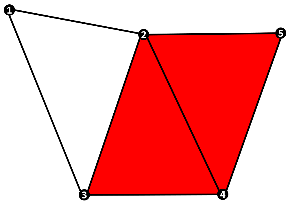

Visual representation of simplicial complex S1

The incidence matrix of order 0 for this is:

[[-1. -1.  0.  0.  0.  0.  0.]
 [ 1.  0. -1. -1. -1.  0.  0.]
 [ 0.  1.  1.  0.  0. -1.  0.]
 [ 0.  0.  0.  1.  0.  1. -1.]
 [ 0.  0.  0.  0.  1.  0.  1.]]

What we see is that if the node is present in the edge subset we add a : +1 if the node is the head in the relationship (tail→head), otherwise a -1. If the node is not found in the subset, we put a zero.

Moving on to Laplacian Matrices

what is it really though?

In the same way, we can generalize different components of rank n in the structure on the basis of their common n+1 rank element. For example, in the edge subset {2,3} if we want to find what other edges are like it—i.e., share a same face or any other parent property—we use laplacians.

A better way to imagine this is going through each rank laplacian and slowly building up the idea.

still don't get it?

Up Laplacians

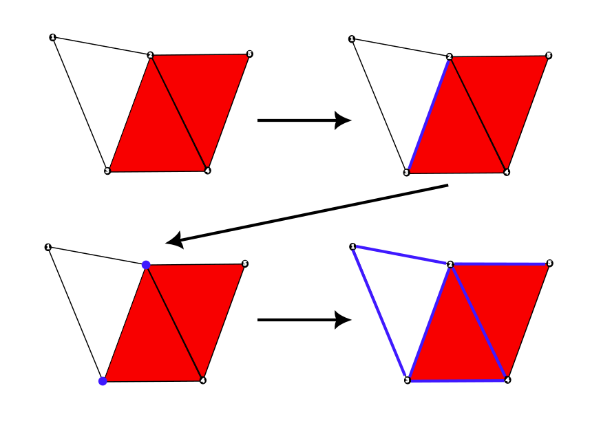
Rank 0 Up Laplacian Relation

General Idea : If any 2 nodes have a shared edge between them.

As a small excercise, take the node 1 in the above defined simplicial structure and look out for its incident edges. From there, find what other nodes are those edges incident to. In our case, the edges are [1,2] and [1,3] and the consequent nodes from them are {1},{2},{3} that share a common property of edges.

Mathematically, this is done by either doing the matrix multiplication of the already found rank 0 incidence matrix with its transpose or doing the subtraction of adjacency matrix from the degree matrix.

finding the up laplacian

L₀ =

[[ 2. -1. -1.  0.  0.]
 [-1.  4. -1. -1. -1.]
 [-1. -1.  3. -1.  0.]
 [ 0. -1. -1.  3. -1.]
 [ 0. -1.  0. -1.  2.]]

Here, the diagonal elements have a weight due to them being the degree of that specific node. Another interesting property of this matrix is that the sum of each row is 0, leading to more useful things like graph clustering and partitioning.

Also, laplacians are used in diffusion models for finding out what amount of values should be transmitted between neighborhood nodes. This wouldn't work out if it didn't sum up to zero (law of conservation required).

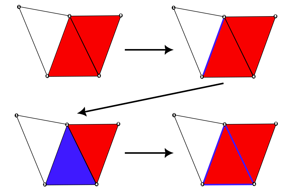
Rank 1 Up Laplacian Relation

If any 2 shared edges have a shared face between them.

Extending this concept over to an even higher rank: to get the edges that share a common face/form the sides of a triangle (a simple 2-d simplex).

However, in a normal graph, the highest laplacian rank we can achieve is 2 as there are no other higher ranked simplexes existing in the structure.

Down Laplacians

fidning down laplacians

• Rank 1 down laplacians relation - if any 2 edges have a shared node
• Rank 2 down laplacians relation - if any 2 faces have a shared edge

              [[ 3. -1.]
              [-1.  3.]]
            

Just like in up laplacians we had an upper bound condition of limiting to rank 2, similarly no rank 0 down laplacians can exist for the same reasons of no simplex of -1 rank being present in the structure.

Hodge Laplacians

Add both the up and down laplacians and you get the hodge laplacian, thereby in a sense seeing the whole structure of graph in all the ways possible, but remember that with the exception of down in rank 0 and up in rank. The resulting laplacian matrix here is a diagonal matrix with the orientations cancelling each other out to produce zeros in the non diagonal elements.

              [[ 3. -1.]
              [-1.  3.]]
            

How Multiplying Incident Matrices Gives Laplacian?

You might wonder how multiplying the matrix that captures whether an element exists in a subset with itself can lead to extracting relationship between elements using a higher dimension as base. For starters, there's this amazing response that you can read on general laplacian operators.

From incidence matrices to laplacians

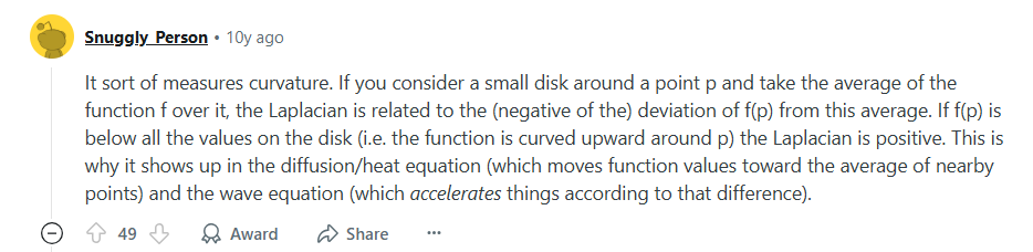
In graph laplacians at the same time when we multiply B·Bᵀ, the Bᵀ is doing the difference operation—i.e., finding the difference between the values at i and j → f[i] - f[j]—and then when it is multiplied with B, which penalizes/awards the deviation from the average by multiplying our terms with ±1.

The laplacian operation on a function f at node i can be expressed as:

(Lf)[i] = deg(i) · f[i] - ∑_{j∼i} f[j]